Chapter 15 Final Project Exercise

* If you would like to know the answers to the questions in this exercise, then you can take this course in Leanpub.

This exercise has been generated to practice everything you have learned in this course set.

15.0.1 GitHub Setup

To get started, you’ll want to go to GitHub and start a new repository:

Call this repository final_project.
Add a short description
Check the box to “Initialize this repository with a README.
Click Create Repository

Once the repository has been created, Click on Clone or download and copy the “Clone with HTTPS” link provided. You’ll use this to clone your repo in RStudio Cloud.

Note: If you’re stuck on this, these steps were covered in detail in an earlier course: Version Control. Refer to the materials in this course if you’re stuck on this part of the project.

15.0.2 RStudio Cloud Setup

Go to the Cloud-based Data Science Space on RStudio Cloud
Click on the “Projects” tab at the top of the workspace
Make a copy of the project: final_project

In this project you should see a final_project.Rmd file. You’ll use this to get started working on your project!

Note: If you try to Knit this document at this time, you will get an error because there is code in this document that has to be edited (by you!) before it will be able to successfully knit!

To start using version control, you’ll want to clone the GitHub repository you just created into this workspace. To do so, go to the Terminal and clone your project into this workspace.

A new directory with the name of your GitHub repository should now be viewable in the Files tab of RStudio Cloud. You are now set up to track your project with git.

15.0.3 Data Science Project Setup

As discussed previously, you’ll want all your data science projects to be organized from the very beginning. Let’s do that now!

First, use cd to get yourself into the directory of your GitHub Project.

Once in the correct directory, use mkdir in the terminal to create folders with the following structure:

- data/
  - raw_data/
  - tidy_data/
- code/
  - raw_code/
  - final_code/
- figures/
  - exploratory_figures/
  - explanatory_figures/
- products/
  - writing/

Now that your directories are set up you’ll want to use the Terminal (or ‘More’ drop-down menu in the Files tab) to move (mv) the final_project.Rmd file into code/raw_code in your version controlled repository**. This ensures that your code file and raw data are in the correct directory.

Once the .Rmd document is in the correct folder, you’ll want to change the author of this document to your name at the top of the .Rmd document (in the YAML). Save this change before moving to the next step.

Note: If you’re stuck on this, these steps were covered in detail in an earlier course: Organizing Data Science Projects. Refer to the materials in this course if you’re stuck on this part of the project.

15.0.4 Pushing to GitHub

You’ll want to save changes to your project regularly by pushing them to GitHub. Now that you’ve got your file structure set up and have added a code file (.Rmd), it’s a good time to stage, commit, and push these changes to GitHub. Do so now, and then take a long on GitHub to see the changes on their website!

Note: If you’re stuck on this, these steps were covered in detail in an earlier course: Version Control. Refer to the materials in this course if you’re stuck on this part of the project.

15.0.5 The Data

The American Time Use Survey (ATUS) is a time-use survey of Americans, which is sponsored by the Bureau of Labor Statistics (BLS) and conducted by the the U.S. Census Bureau. Respondents of the survey are asked to keep a diary for one day carefully recording the amount of time they spend on various activities including working, leisure, childcare, and household activities. The survey has been conducted every year since 2003.

Included in the data are a number of demographic variables (such as respondents’ age, sex, race, marital status, and education) as well as detailed income and employment information for each respondent. While there are some slight changes to the survey each year, the main questions asked stay the same. You can find the data dictionaries, which provide information about the variables included for each year’s survey at https://www.bls.gov/tus/dictionaries.htm.

15.0.6 Accessing the Data

There are multiple ways to access the ATUS data; however, for this project, you’ll get the raw data directly from the source. The data for each year can be found at https://www.bls.gov/tus/#data. Once there, there is an option of downloading a multi-year file, which includes data for all of the years the survey has been conducted, but for the purposes of this project, let’s just look at the data for 2016. Under Data Files, click on American Time Use Survey--2016 Microdata files.

American Time Use Survey

You will be brought to a new screen. Scroll down to the section 2016 Basic ATUS Data Files. Under this section, you’ll want to click to download the following two files: ATUS 2016 Activity summary file (zip) and ATUS-CPS 2016 file (zip).

Download Data Files

ATUS 2016 Activity summary file (zip) contains information about the total time each ATUS respondent spent doing each activity listed in the survey. The activity data includes information such as activity codes, activity start and stop times, and locations.
ATUS-CPS 2016 file (zip) contains information about each household member of all individuals selected to participate in the ATUS.

Once they’ve been downloaded, you’ll need to unzip the files. Once unzipped, you will see the dataset in a number of different file formats including .sas, .sps, and .dat files. We’ll be working with the .dat files.

15.0.7 Loading the Data into R

To use the data in RStudio Cloud, you’ll have to upload the two .dat files (atuscps_2016.dat and atussum_2016.dat) into RStudio Cloud. Make sure the data are stored in the raw_data folder.

Once uploaded into the correct folder, you’ll be able to load the data in, You’ll do this by first running the setup chunk in the final_project.Rmd file and then by running the code in the atus-data code chunk. This will create an object called atus.all.

How many observations are in the dataset?

15.0.8 Analyze the Data

Now that we’ve got the data in RStudio Cloud, let’s get to work!

15.0.8.1 Exploratory Data Analysis

Once the data have been read in, explore the data, adding your initial exploratory code to the initial-exploration code chunk in final_project.Rmd. Then, answer the following questions:

You can find data dictionaries (also called codebooks) at https://www.bls.gov/tus/atuscpscodebk16.pdf for the CPS data and at https://www.bls.gov/tus/atusintcodebk16.pdf for the rest of the variables. Using this data dictionary is very important as a lot of the information about the variables in the data and how they are coded can be found here. By looking at the variables in the data frame atus.all, we see that there are a lot of variables that start with t followed by a 6-digit number. These variables capture the total number of minutes each respondent spent doing each activity. The link https://www.bls.gov/tus/lexiconwex2016.pdf lists all the activity codes. Using the information in that file, what column is associated with the activity “playing computer games”? Your answer should start with t and then a 6-digit number that combines the major category, the 2nd tier, and the 3rd tier of the activity. For instance, if major category in equal to 05, second tier is equal to 03, and third tier is equal to 01, then your answer should be t050301.
In the data, the variable t010101 contains the total number of minutes each respondent spent doing activity 010101 which is “sleeping” and the variable t010102 contains the total number of minutes each respondent spent doing activity 010102, “sleeplessness.” Find the variable associated with “Socializing and communicating with others.” How much time, on average, does a person in the sample spend on “Socializing and communicating with others”? Again, The link https://www.bls.gov/tus/lexiconwex2016.pdf lists all the activity codes.

Find the activity code that is associated with “Caring For & Helping HH Children”. This is a level 2 activity so we need to add all the variables that start with t0301. Create a column in the data frame atus.all called CHILDCARE that is the sum of all the columns that start with t0301. Here, you’ll have to change the code chunk creating-childcare-var.

Move on to the code chunk called childcare-density-plot and write code in ggplot2 to plot the density function of the variable CHILDCARE.

From the data dictionary, what is the variable that shows the gender of the respondent?
From the data dictionary, the variable that represents the gender of the respondents can one of take two values, 1 or 2. Which gender group does 1 represent?

15.0.8.2 Inferential Data Analysis

We are going to answer whether women or men spend more time with their children. Start by grouping individuals by their gender and calculate the average time men and women spend with their children. Use the code chunk gender-analysis in the .Rmd file. Note that you should replace FUNCTION in order to calculate the average of the variable CHILDCARE.

Men and women are different in the amount of time they spend with their children. Which group spends more time, men or women?

Use the table() function to look at the variable TRDPFTPT which shows whether the person works full time or part time. You will notice that the variable also takes the value -1. This is probably due to non-response or other data collection reasons. Replace these values with NA in your data so they don’t affect your analysis. Use the code chunk replacing-na for doing this and add your commands there.

How many NAs are in the variable now?

Now, we are going to explore what factors affect time spent with children. We are going to answer questions like:

Do younger parents spend more time with their children?
Do richer people spend more time with their children compared to poorer people?
Do married couples spend more time with their children compared to single parents?
Do full-time workers spend more time with their children compared to part-time workers?

Compare each of these relationships and present your results in a table or a graph. You can do this by first finding these variables from the data dictionary. Add your code in the code chunk exploratory-analysis in the .Rmd file. Make sure that in your analysis, you limit your data to those who have at least one child (18 or younger) in the household. The variable for the number of children (18 or younger) in the household is TRCHILDNUM. Use the data frame atus.all that you previously created and again limit your data to those who have at least one child (18 or younger) in the household. The variable for income is HEFAMINC. Other variables are easy to find from the data dictionary.

In the exercise above, we looked at bilateral (two-way) relationships. For instance, we looked at how income and time spent with children are related. You have learned in this course, however, that other confounding variables can be a source of bias in your analysis. For instance, the effect of income on time spent with children can be biased by the number of children a person has. Maybe richer people spend less time because they have fewer children. It’s much better to look at the relationship of all relevant variables associated with time spent with children together. Run a linear regression of marital status, age, sex, number of children (18 or younger), earnings, and full-time versus part-time status. Add your code in the reg-analysis code chunk. Remember to limit the sample to those who have at least one child (18 or younger) in the household. Also make sure to to change the values of the variable TRDPFTPT that are -1 to NA.

What is the coefficient on gender now?
In the regression, the coefficient on the variable age means how much time spent with children changes if age increases by 1. Based on your results, what’s the difference in minutes spent with children between two people with 10 years of age difference?

In the next few questions, we are going to see whether time spent on different activities varies by age. However, we will only consider activities at the major category levels. There are 18 major categories in the data including personal care, household activities, caring for & helping household members, etc. Because each activity column in the data is at the 3rd tier, we will need to start by suming columns at the activity major categories levels. Save the resulting data frame as df.wide. Use code chunk activity-cats in the .Rmd file for this part.

What activity group do people spent, on average, most time on?
Which is the second most time consuming activity for the respondents?
What is the maximum time a person in our sample spends time on “Work & Work-Related Activities”?

Convert the data from wide to long using the package of your choice and save the data frame as df.long. Use the code chunk wide-to-long for this purpose. Make sure your key variable is called ACTIVITY and your value variable is called MINS.

Now, group the data frame you created in the previous step by activity type (ACTIVITY) and age (TEAGE). Calculate the average time for each age group and call it AVGMINS. In ggplot2, plot AVGMINS against TEAGE for each category (multiple panels). Type your code in the code chunk age-activity. Label each panel in your graph with the appropriate activity name.

For which categories does the average time spent vary by age?
Based on the graph, what is true about the activity category 5 (Work & Work-Related Activities)?
- 65-year olds work the most.
- Young, middle-aged, and old workers spend more or less the same number of hours working.
- Young people work more than middle-aged people.
- Middle aged people work the most compared to younger and older people.
Based on the graph, what is true about the activity category 12 (Socializing, Relaxing, and Leisure)?
- Older people spend more time socializing.
- Middle-aged people are the most social.
- Younger people socialize more than older people.
- Young people are the most social.

15.0.8.3 Data Visualization

Finally, in this last step, we are going to create a graph that shows how different income groups spend time doing each activity. The graph is based on Henrik Lindberg’s data visualization posted here. The only difference is that we are only looking at the 18 major activity categories. Use the long data that you created in the previous section and make the graph as close as possible to the graph by Henrik Lindberg. Type your code in the code chunk activity-income.

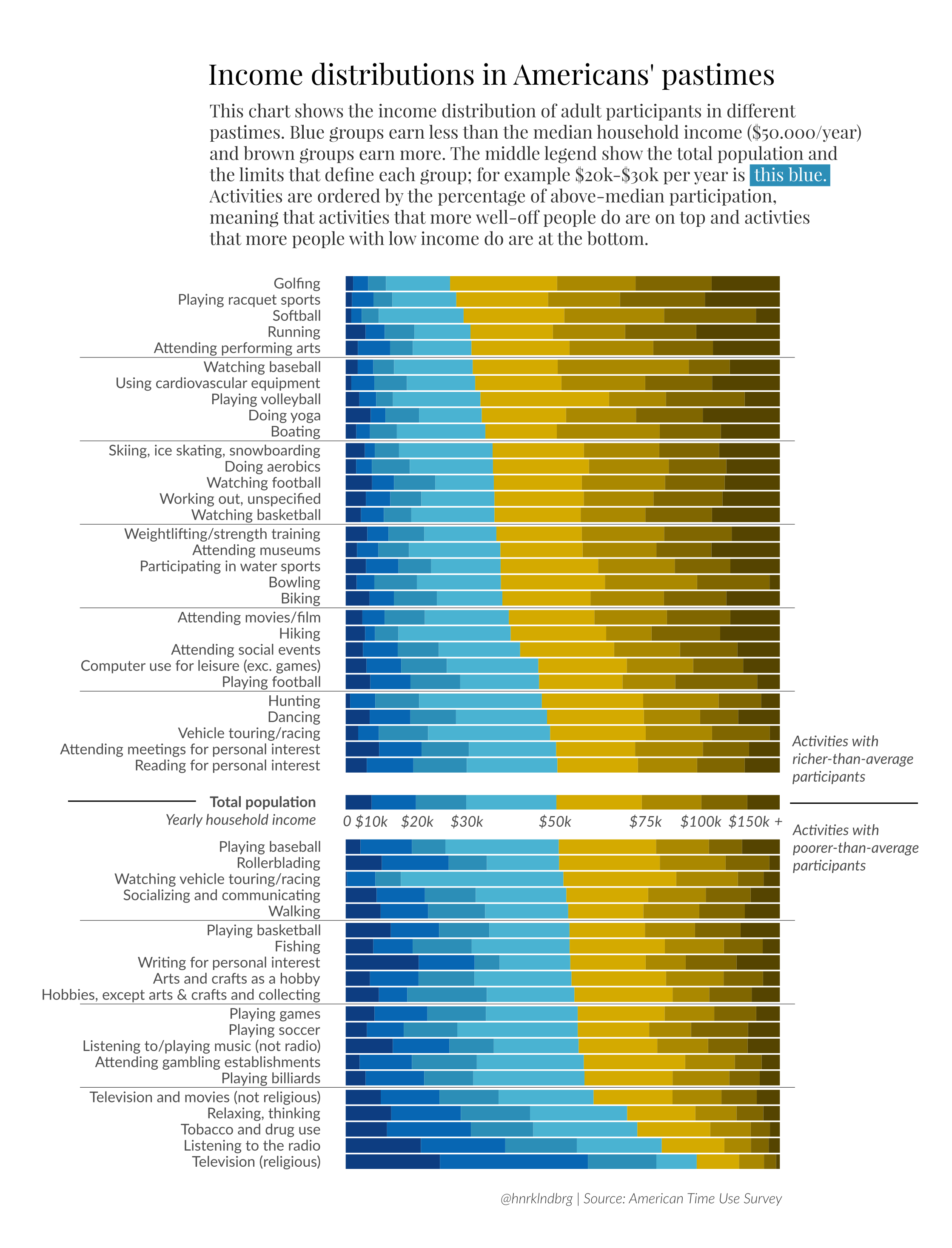
15.0.8.4 Save the Plot

Once you’ve worked through this code chunk and have a plot that looks very similar to the plot in the original publication (and that you see above), you’ll want to use ggsave() to save this plot to figures/explanatory_figures. Save this figure as “activity-income.png”. Do this using the partial code in the code chunk save-plot.

15.0.9 Add Markdown Text to .Rmd

Before finalizing your project you’ll want be sure there are comments in your code chunks and text outside of your code chunks to explain what you’re doing in each code chunk. These explanations are incredibly helpful for someone who doesn’t code or someone unfamiliar to your project.

Note: If you’re stuck on this, these steps were covered in detail in an earlier course: Introduction to R. Refer to the R Markdown lesson in this course if you’re stuck on this part (or the next part) of the project.

15.0.10 Knit your R Markdown Document

Last but not least, you’ll want to Knit your .Rmd document into an HTML document. If you get an error, take a look at what the error says and edit your .Rmd document. Then, try to Knit again! Troubleshooting these error messages will teach you a lot about coding in R.

15.0.11 A Few Final Checks

A complete project should have:

Completed code chunks throughout the .Rmd document (your RMarkdown document should Knit without any error)
README.md text file explaining your project
Comments in your code chunks
Answered all questions throughout this exercise.

15.0.12 Final `push` to GitHub

Now that you’ve finalized your project, you’ll do one final push to GitHub. add, commit, and push your work to GitHub. Navigate to your GitHub repository, and answer the final question below!

Note: If you’re stuck on this, these steps were covered in detail in an earlier course: Version Control. Refer to the materials in this course if you’re stuck on this part of the project.

Congrats on finishing your Final Project!!

{/exercise}

Chapter 15 Final Project Exercise

15.0.1 GitHub Setup

15.0.2 RStudio Cloud Setup

15.0.3 Data Science Project Setup

15.0.4 Pushing to GitHub

15.0.5 The Data

15.0.6 Accessing the Data

15.0.7 Loading the Data into R

15.0.8 Analyze the Data

15.0.8.1 Exploratory Data Analysis

15.0.8.2 Inferential Data Analysis

15.0.8.3 Data Visualization

15.0.8.4 Save the Plot

15.0.9 Add Markdown Text to .Rmd

15.0.10 Knit your R Markdown Document

15.0.11 A Few Final Checks

15.0.12 Final push to GitHub

15.0.12 Final `push` to GitHub